How To Make A Cashier Count Chart In Excel / Cashier Resume Sample Writing Guide Resume Genius - Next, sort your data in descending order.

How To Make A Cashier Count Chart In Excel / Cashier Resume Sample Writing Guide Resume Genius - Next, sort your data in descending order.. The new feature was announced on the microsoft office blog in display empty cells, null (#n/a) values, and hidden worksheet data in a chart. On a mac, you'll instead click the design tab, click add chart element, select chart title, click a location, and type in the graph's title. While most of the charts in excel are easy to create, pie charts are even easier. Click the insert line or area chart icon. We will input the data as shown in figure 2 into the excel sheet;

Create a combo chart with a secondary axis. Navigate to the insert tab. While most of the charts in excel are easy to create, pie charts are even easier. On a mac, you'll instead click the design tab, click add chart element, select chart title, click a location, and type in the graph's title. Select data for the chart.

Cash Register Report Daily Cash Register Summary Help For Flare Online Accounting Software Users from support.flareapps.com

Select all of the data in your table, including the header row and column. Select a chart on the recommended charts tab, to preview the chart. The select data source window will open. Change the horizontal axis labels. Excel rolling chart creating reports on a regular schedule is a common task for the business excel user. From the insert tab on the ribbon, click on the icon that shows a column chart. In a recent build of excel 2016, the behavior of #n/a in a chart's values has changed. Select the data range and click table under insert tab, see screenshot:

First, select a number in column b.

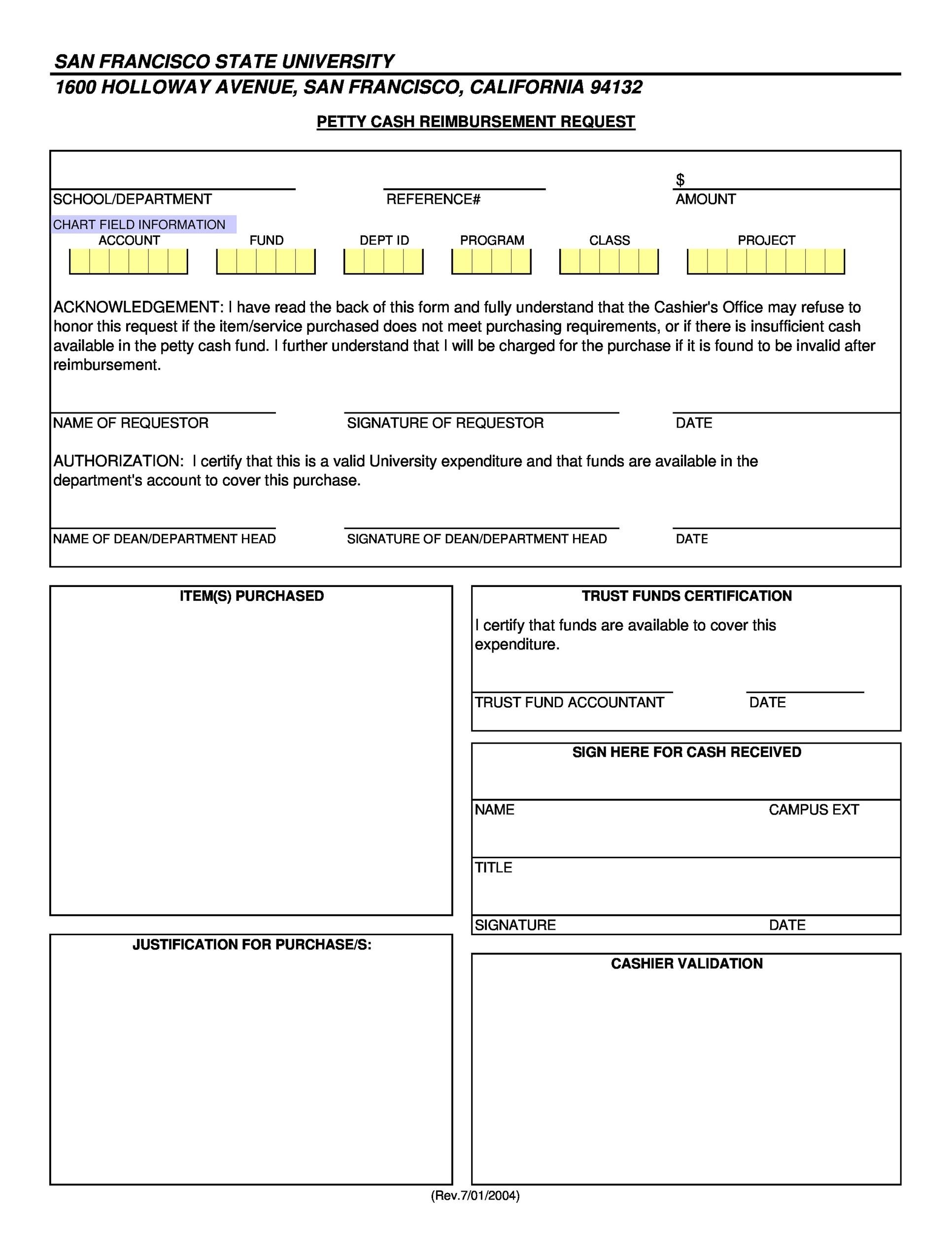
In this video tutorial, you'll see how to create a simple pie graph in excel. First, add the pointer values into the existing chart. Select the data range and click table under insert tab, see screenshot: The cash count sheet can be used to total the amount of cash counted and compares this to the cash book value, and record any difference between the two. We will open a new excel sheet; Select insert from the menu. Select the data to include on the chart. Select the column category and 3 patient's quantity of conception. Let's start with the good things first. With the chart selected, click the design tab. Select the see all charts option and get more charts types. Also remember to enter a name for series name. To create a vertical histogram, you will enter in data to the chart.

To create a vertical histogram, you will enter in data to the chart. This would insert a cluster chart with 2 bars (as shown below). Highlight all the data from the chart inputs table (a9:j12). Click the insert statistic chart button to view a list of available charts. This method works with all versions of excel.

40 Petty Cash Log Templates Forms Excel Pdf Word á… Templatelab from templatelab.com

In excel 2007, 2010 or 2013, you can create a table to expand the data range, and the chart will update automatically. A simple chart in excel can say more than a sheet full of numbers. In that case, an excel filter can come in handy when you want to see your sales performance in a selected region, based on a particular age group. This method works with all versions of excel. In select data source dialog, click on add button and select the range that contains width, start, end for the series values input. Change the horizontal axis labels. Click the insert statistic chart button to view a list of available charts. Select insert > recommended charts.

I recommend you watch the video as it will likely help you to follow along.

To create a line chart, execute the following steps. Next, sort your data in descending order. Select a black cell, and press ctrl + v keys to paste the selected column. In excel 2013, you can quickly show a chart, like the one above, by changing your chart to a combo chart. Select insert > recommended charts. Let's start with the good things first. The cash count sheet can be used to total the amount of cash counted and compares this to the cash book value, and record any difference between the two. To create a chart, follow these steps: Plot #n/a as blank in excel charts. You don't need to worry a lot about customization as most of the times, the default settings are good enough. When you have a lot of numeric data on a microsoft excel worksheet, using a chart can help make more sense out of the numbers. On the data tab, in the sort & filter group, click za. Here are the steps to create the chart.

In the charts group, click on the 'insert column or bar chart' icon. Change the horizontal axis labels. You can select the data you want in the chart and press alt + f1 to create a chart immediately, but it might not be the best chart for the data. Click that rectangle (you may need to move or hide the text pane) and type the name of that person. Select the data to include on the chart.

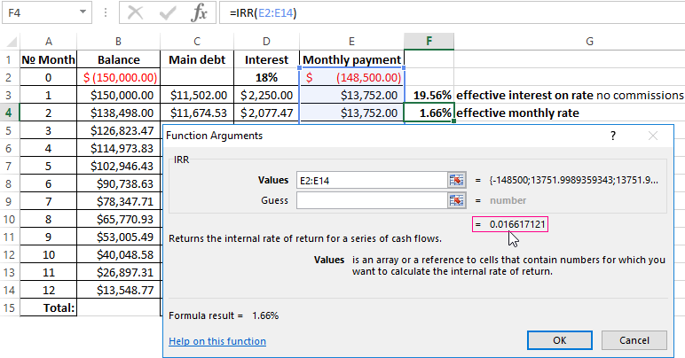
Calculation Of The Effective Interest Rate On Loan In Excel from exceltable.com

Select data for the chart. In excel 2007, 2010 or 2013, you can create a table to expand the data range, and the chart will update automatically. Change the horizontal axis labels. It is now possible to make excel plot #n/a values as empty cells. On the data tab, in the sort & filter group, click za. The cash count sheet can be used to total the amount of cash counted and compares this to the cash book value, and record any difference between the two. We will input the data as shown in figure 2 into the excel sheet; Also remember to enter a name for series name.

We will click on anywhere on the data, click on the insert tab, and click on table as shown in figure 3;

We will input the data as shown in figure 2 into the excel sheet; If you don't have excel 2016 or later, simply create a pareto chart by combining a column chart and a line graph. Excel filters can also be useful when you want to create a smaller group before plotting your excel data on a chart. Click on the small down arrow icon. On the insert tab, in the charts group, click the line symbol. You don't need to worry a lot about customization as most of the times, the default settings are good enough. The shape (which is a rectangle) at the top of the chart is the head of the organization. To create a vertical histogram, you will enter in data to the chart. We will open a new excel sheet; Change the chart type of one or more data series in your chart (graph) and add a secondary vertical (value) axis in the combo chart. Tallying certain criteria in your excel 2010 spreadsheet totals the number of times the criteria appears in that document. Change the horizontal axis labels. Select data for the chart.

Cari Blog Ini

elpozodelamazorca